
Word Cloud: A tool of visualization, communication and insights
Published:
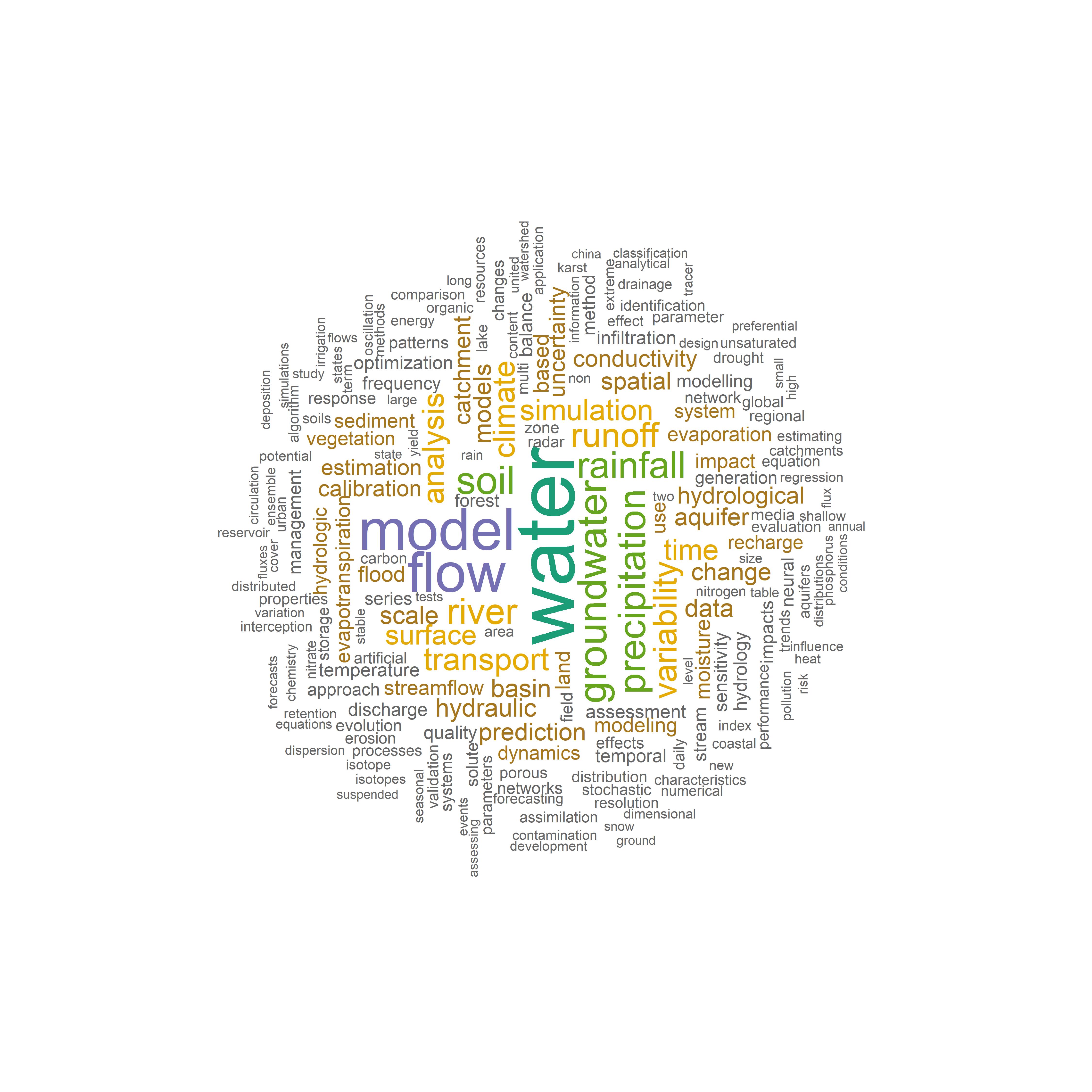
A word cloud is a collection or cluster of words described in different sizes. The larger the word appears, the more times it is mentioned in a given text, and the more important it is.
How it works?
A word cloud (also called a tag cloud) works in a simple way: the more a specific word appears in a text data source (such as a speech, blog post or database), the bigger size it appears in the word cloud.
Reasons why you should use word clouds
Word clouds are killer visualisation tools. They present text data in a simple and clear format, that of a cloud in which the size of the words depends on their respective frequencies. As such, they are visually nice to look at as well as easy and quick to understand.
Word clouds are great communication tools. They are incredibly handy for anyone wishing to communicate a basic insight based on text data — whether it’s to analyse a speech, capture the conversation on social media or report on customer reviews.
Word clouds are insightful. Visually engaging, word clouds allow us to draw several insights quickly, allowing for some flexibility in their interpretation. Their visual format stimulates us to think and draw the best insight depending on what we wish to analyse.
Text mining using Python
WOS_Crawler is a crawler of Web of Science:
- Supported crawling approaches:
- Support GUI of crawling (crawl_by_gui)
- Support crawling the search results of any legal advanced search style (crawl_by_query)
- Support crawling a given journal list to crawl all the articles in the journal (crawl_by_journal)
- Supported input & output types:
- Support the selection of target document types, such as Article, Proceeding paper, etc.
- Support a variety of storage formats for crawling results, such as Plain text, Bibtex, HTML, etc. Plain text is recommended for the fastest parsing speed
- Support for parsing and importing crawling results into the database (currently supporting Plain text, Bibtex, and XML format parsing and importing). In addition to basic document information (titles, abstracts, keywords, citations, etc.), the parsing data items also include Author institution, fund, classification, references and other information
More details refer to:
https://blog.csdn.net/tomleung1996/article/details/86627443
https://github.com/tomleung1996/wos_crawler
Prepare for WOS_Crawler
### In this example, setup crawlering Journal of Hydrology paper from 2001 to 2021

#journal_list_water.txt - J HYDROL

#select the crawling approach
if __name__ == '__main__':
    # journal based
    crawl_by_journal(journal_list_path='../input/journal_list_water.txt',
                     output_path='../output', output_format='fieldtagged', document_type='Article')

    # query based
    # crawl_by_query(query='TS=(solid waste) AND PY=(1900-1978)',
    #                output_path='../output', output_format='fieldtagged', document_type='Article', sid='E5gsGHmjPtA2AxeNeM6')

    # GUI based
    # crawl_by_gui()
    # pass
Workflow
Load necessary packages
library(wordcloud)
library(wordcloud2)
library(RColorBrewer)

library(tm) # for text mining
library(dplyr)
library(readr)
library(ggplot2)
Text analysis
#the folder where downloaded text are
filepath <- "./data/journal"

file.list <- list.files(filepath,full.names=TRUE)

file.list.JoH <- file.list[grep("J HYDROL",file.list)]


tmp.title=tmp.keyword <- NULL
for (tmp.file in file.list.JoH) {

  file.txt <- sapply(list.files(tmp.file,full.names=TRUE), function(path) readLines(path))

  tmp.title <- c(tmp.title, sapply(file.txt, function(txt) txt[!is.na(stringr::str_extract(txt, "TI"))]))
  tmp.keyword <- c(tmp.keyword, sapply(file.txt, function(txt) txt[!is.na(stringr::str_extract(txt, "DE"))]))

}


text.keyword <- do.call(rbind, tmp.keyword)
text.title <- do.call(rbind, tmp.title)

# Clean the text data
# gsub("https\\S*", "", text)
# gsub("@\\S*", "", text)
# gsub("  title = ", "", text)
# gsub("[\r\n]", "", text)
# gsub("[[:punct:]]", "", text)
text.title <- gsub("‐", " ", text.title)

text.title.n <- iconv(text.title, "UTF-8", "UTF-8",sub='')
text1 <- gsub("\\}.*", "}", gsub(".*\\{", "{", text.title.n))

# Create a corpus
docs <- Corpus(VectorSource(text1))

# Clean the text data
docs <- docs %>%
  tm_map(removeNumbers) %>%
  tm_map(removePunctuation) %>%
  tm_map(stripWhitespace)
docs1 <- tm_map(docs, content_transformer(tolower))
docs2 <- tm_map(docs1, removeWords, stopwords("english"))

# Create a document-term-matrix
dtm <- TermDocumentMatrix(docs2)
matrix <- as.matrix(dtm)
words <- sort(rowSums(matrix),decreasing=TRUE)

df <- data.frame(word = names(words),freq=words)
summary(df)
head(df)
Word frequency analysis
ggplot(df[df$freq>quantile(df$freq,0.99),]) +
  geom_col(aes(x=word, y=freq)) +
  theme_bw()+
  theme(axis.text.x = element_text(angle = 90, vjust = 0.5, hjust=1))
Word Cloud generation
###with wordcloud package
set.seed(2021-04-28) # for reproducibility

df1 <- df
head(df1)

###remove unwanted words manually
df.text1 <- df1[!(df1$word %in% c("–","using","and","for","of")),]

max.words <- quantile(nrow(df), 0.01)
max.words <- 200
wordcloud(words = df.text1$word, freq = df.text1$freq, min.freq = 1, max.words=max.words, random.order=FALSE,
          rot.per=0.35, colors=rev(brewer.pal(8, "Dark2")))
###with wordcloud2 package
set.seed(1234) # for reproducibility

df2 <- df
head(df2)

df.text2 <- df2[!(df2$word %in% c("–","using","and","for","of")),]

wordcloud2(data=df.text2, size=0.35, color='random-dark',shape = 'circle',ellipticity=1)
wordcloud2(data=df.text2, size=0.35, color='random-dark',shape = 'square',ellipticity=1)
wordcloud2(data=df.text2, size = 0.35, shape = 'pentagon',ellipticity=1)